TimescaleDB Alternatives for Multimodal Data

TimescaleDB is an open-source time-series database optimized for fast ingest and complex queries. It is engineered up from PostgreSQL and offers the power, reliability, and ease-of-use of a relational database, combined with the scalability typically seen in NoSQL systems. It is particularly suited for storing and analyzing things that happen over time, such as metrics, events, and real-time analytics.

Since TimescaleDB is based on PostgreSQL, it supports blob data and can be used to store a history of unstructured data such as images, binary sensor data, or large text documents. In this article, we will use the database as a time-series blob storage and compare its performance with ReductStore, which is designed specifically for this use case.

TimescaleDB and ReductStore both have Python Client SDKs. We'll create simple Python functions to read and write data, then compare performance with different blob sizes. To repeat these benchmarks on your own machine, use this repository.

Read/Write Blob Data With TimescaleDB

Since TimescaleDB is a part of PostgreSQL, you can use the psycopg adapter for Python to manage the database and stream the data. In this section, we initialize the TimescaleDB extension, recreate the benchmark database, and create a table for our blob data. Once the table is prepared, we write a chunk of binary data with the current time BLOB_COUNT times. To speed up the writing process, we use the execute_values function from the psycopg2.extras module and write data in batches of BATCH_MAX_RECORDS=80 records or BATCH_MAX_SIZE=8M bytes.

import psycopg2
from psycopg2.extensions import ISOLATION_LEVEL_AUTOCOMMIT

BLOB_SIZE = 1000_000
BATCH_MAX_SIZE = 8_000_000
BATCH_MAX_RECORDS = 80

BLOB_COUNT = min(1000, 1_000_000_000 // BLOB_SIZE)

CHUNK = random.randbytes(BLOB_SIZE)

HOST = "localhost"
CONNECTION = f"postgresql://postgres:postgres@{HOST}:5432"

def setup_database():
    con = psycopg2.connect(CONNECTION)
    con.set_isolation_level(ISOLATION_LEVEL_AUTOCOMMIT)
    cur = con.cursor()
    cur.execute("CREATE EXTENSION IF NOT EXISTS timescaledb CASCADE;")
    cur.execute(f"DROP DATABASE IF EXISTS benchmark")
    cur.execute(f"CREATE DATABASE benchmark")
    con.commit()
    con.close()

def write_to_timescale():
    setup_database()

    with psycopg2.connect(CONNECTION + "/benchmark") as con:
        with con.cursor() as cur:
            cur.execute(
                f"""CREATE TABLE data (
                       time TIMESTAMPTZ NOT NULL,
                       blob_data BYTEA NOT NULL);
                """
            )
            cur.execute("SELECT create_hypertable('data', by_range('time'))")
            con.commit()

            count = 0
            values = []
            for i in range(0, BLOB_COUNT):
                values.append((datetime.now(), psycopg2.Binary(CHUNK)))
                sleep(0.000001)  # To avoid time collisions
                count += BLOB_SIZE

                if len(values) >= BATCH_MAX_RECORDS or len(values) * BLOB_SIZE >= BATCH_MAX_SIZE:
                    psycopg2.extras.execute_values(
                        cur,
                        "INSERT INTO data (time, blob_data) VALUES %s;",
                        values,
                    )
                    values = []


            if len(values) > 0:
                psycopg2.extras.execute_values(
                    cur,
                    "INSERT INTO data (time, blob_data) VALUES %s;",
                    values,
                )

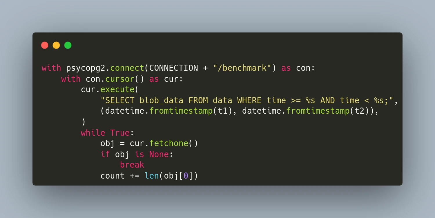
Now we need to create a function to read all the blobs from the table, it is quite easy, and we need only one SELECT request:

def read_from_timescale(t1, t2):
    count = 0
    with psycopg2.connect(CONNECTION + "/benchmark") as con:
        with con.cursor() as cur:
            cur.execute(
                "SELECT blob_data FROM data WHERE time >= %s AND time < %s;",
                (datetime.fromtimestamp(t1), datetime.fromtimestamp(t2)),
            )
            while True:
                obj = cur.fetchone()
                if obj is None:
                    break
                count += len(obj[0])

    return count

As you can see, working with Timescale is quite easy if you are familiar with any SQL database. However, you may notice that we should put the whole blob into the INSERT request. This could cause a performance problem for large blobs because we have to allocate the memory for the request string instead of sending it in chunks.

Let’s see how you can write and read data with ReductStore.

Read/Write Blob Data With ReductStore

With ReductStore, you can write and read data without using SQL requests, simply by utilizing the asynchronous API. Additionally, if you need to handle large blobs, you can stream them in chunks without loading them into memory. In this example, we also write data in batches to speed up the process for relatively small blobs.

from reduct import Client as ReductClient

async def write_to_reduct():async def write_to_reduct():
    async with ReductClient(
        f"http://{HOST}:8383", api_token="reductstore"
    ) as reduct_client:
        count = 0
        bucket = await reduct_client.get_bucket("benchmark")
        batch = Batch()
        for i in range(0, BLOB_COUNT):
            batch.add(timestamp=datetime.now().timestamp(), data=CHUNK)
            await asyncio.sleep(0.000001)  # To avoid time collisions
            count += BLOB_SIZE

            if  batch.size >= BATCH_MAX_SIZE or len(batch) >= BATCH_MAX_RECORDS:
                await bucket.write_batch("data", batch)
                batch.clear()

        if len(batch) > 0:
            await bucket.write_batch("data", batch)

        return count

async def read_from_reduct(t1, t2):
    async with ReductClient(
        f"http://{HOST}:8383", api_token="reductstore"
    ) as reduct_client:
        count = 0
        bucket = await reduct_client.get_bucket("benchmark")
        async for rec in bucket.query("data", t1, t2):
            count += len(await rec.read_all())
        return count

Benchmarks

After establishing our read/write functions, we can start writing our benchmarks.

if __name__ == "__main__":
    print(f"Chunk size={BLOB_SIZE / 1000_000} Mb, count={BLOB_COUNT}")
    ts = time.time()
    size = write_to_timescale()
    print(f"Write {size / 1000_000} Mb to TimescaleDB: {BLOB_COUNT / (time.time() - ts)} req/s")

    ts_read = time.time()
    size = read_from_timescale(ts, time.time())
    print(f"Read {size / 1000_000} Mb from TimescaleDB: {BLOB_COUNT / (time.time() - ts_read)} req/s")

    loop = asyncio.new_event_loop()
    ts = time.time()
    size = loop.run_until_complete(write_to_reduct())
    print(f"Write {size / 1000_000} Mb to ReductStore: {BLOB_COUNT / (time.time() - ts)} req/s")

    ts_read = time.time()
    size = loop.run_until_complete(read_from_reduct(ts, time.time()))
    print(f"Read {size / 1000_000} Mb from ReductStore: {BLOB_COUNT / (time.time() - ts_read)} req/s")

For testing purposes, we need to run the databases. This can easily be done using docker-compose:

version: "3"
services:
  timescale:
    image: timescale/timescaledb:latest-pg14
    ports:
      - "5432:5432"
    environment:
      POSTGRES_USER: postgres
      POSTGRES_PASSWORD: postgres
    volumes:
      - ${PWD}/data/timescale:/var/lib/postgresql/data

  reductstore:
    image: reduct/store:latest
    ports:
      - "8383:8383"
    environment:
      RS_API_TOKEN: reductstore
      RS_BUCKET_1_NAME: benchmark
      RS_BUCKET_1_QUTA_TYPE: FIFO
      RS_BUCKET_1_QUOTA_SIZE: 50TB

    volumes:
      - ${PWD}/data/reductstore:/data

Take note, ReductStore enables the provisioning of any resources with environment variables. In this case, we create a bucket called benchmark with a 50TB quota. Your DevOps team will appreciate it.

Let's set up and run benchmarks:

docker-compose up -d
python3 main.py

Results

The script displays results for the specified BLOB_SIZE and SIZE_COUNT. On my device, which has an NVMe drive, here are the results I obtained:

Chunk Size	Operation	TimescaleDB, blob/s	ReductStore, blob/s	ReductStore, %
1 KB	Write	3124	9322	+198%
	Read	40300	51505	+28%
10 KB	Write	2114	8395	+297%
	Read	10241	42322	+313%
100 KB	Write	491	5026	+924%
	Read	1602	11244	+603%
1 MB	Write	56	898	+1604%
	Read	173	1336	+671%

Based on the benchmark results, ReductStore outperforms TimescaleDB in both write and read operations. The performance difference increases with the blob size, reaching up to 1604% for writing and 671% for reading 1MB blobs. This is due to the fact that ReductStore is optimized for storing and retrieving blobs, while TimescaleDB is designed for structured data and complex queries.

Other Considerations

When we choose a database for storing blob data, we should consider not only performance but also the following factors:

• Retention Policy: ReductStore provides a retention policy based on disk usage, which is crucial when the amount of data stored over time is unpredictable.
• Data Size: ReductStore is more efficient for storing large blobs, while TimescaleDB is better for small blobs.
• Querying: TimescaleDB is better for structured data and complex queries, while ReductStore is more suitable for storing and retrieving blobs with minimal overhead and latency.
• Replication: TimescaleDB replicates data across multiple nodes as exact copies, while ReductStore provides append-only replication, with the ability to filter data based on labels. This could be a part of your data reduction strategy.

When TimescaleDB Is Still the Right Choice

Keep TimescaleDB when your records are structured rows and you ask for them by aggregate. Continuous aggregates, hypertable partitioning and columnar compression are real advantages, and an object store has no equivalent for any of them. TimescaleDB is particularly strong when you want SQL joins and relational data directly alongside the readings, for example against an asset table, a work order or a shift schedule. That is not a job to hand to a blob store.

Keep it when your payloads are small. Under roughly 2 KB of total row size, TOAST never triggers, the value sits inline, and the overhead measured above never appears. One INSERT writes it, one SELECT reads it back, and there is no second system to keep consistent.

The problem starts above that threshold, and the mechanism is worth naming.

Three Kinds of TimescaleDB Alternative

Your problem is analytical scale on structured data. You have billions of numeric rows and the aggregate queries have stopped finishing in time. You want a different SQL engine, not an object store. ClickHouse, QuestDB and InfluxDB sit in this group. A migration keeps the shape of your data and swaps the engine underneath it.

Your problem is size. The rows are fine, but each one carries an image, a waveform or a serialized message, and the database is now mostly payload. You want the payload out of the database. The standard answer is an object store with a metadata table pointing into it. It works, and you own the consistency between the two systems and the retention on both of them. We measured the same workload against S3 style storage in the MinIO comparison.

Your problem is time and modality together. The payloads have to leave the database and you still have to ask for them by time range, by device, by label. This is the physical AI case: several streams of different types and sizes recorded against one clock, large enough that storing the payload directly as database rows becomes inefficient, and not much use without the others. That is what this post benchmarks.

The second problem usually leads teams to use a combination of a bucket and a table. However, we recommend checking the third option first. This is because the metadata table is often where the complexity of synchronisation, retention and consistency accumulates.

The same split shows up against MongoDB and against InfluxDB and MinIO together.

Time-Indexed Storage Is Not a Time Series Database

A physical AI workload records several modalities against one clock. A camera frame, a lidar scan, an audio window, an IMU burst and a row of structured telemetry all belong to the same moment, and they run from a hundred byte row to a multi megabyte frame. The question is not where to put the biggest one. It is what indexes all of them.

Three storage shapes get called on here, and they differ in what the primary index is.

A time series database indexes by timestamp. That is what makes a range query cheap, and it is why TimescaleDB is a reasonable first thing to try. The cost is that the payload has to stay small.

An object store indexes by key. The payload can be any size and any type, which solves the problem the time series database has, and it gives up the index to do it. Time is not a dimension S3 knows about, so you encode it in the key and list a prefix, or you keep a metadata table beside the bucket and join on it. With one modality that is tolerable. With five it is a schema you now own and have to keep correct.

Time-indexed storage keeps the timestamp as the primary index and leaves the payload opaque and unbounded. A record is a timestamp, a blob of any size, and a set of labels. Each modality is its own entry in the same bucket, written against the same clock. Pulling a moment back is a time range across entries rather than a join you wrote yourself.

	Primary index	Payload	Several modalities
Time series database	timestamp	small, structured	one table, one schema
Object store	key string	any size, any type	your naming scheme
Time-indexed storage	timestamp	any size, any type	one entry each, shared clock

ReductStore is the third row. It is not a time series database that accepts binary payloads, and calling it one sets the wrong expectation. There is no continuous aggregate, no hypertable partitioning, no join against an asset table. What it does is keep the timestamp as the index across every modality, at payload sizes a row based database cannot hold.

Retention, SQL and Schema

The first decision is whether to move the payload out. The second is what you can do with it once it is out, and this is where a time-indexed store differs from a simple bucket.

• Lifecycle policies run as background tasks on a bucket. They delete old records or compress persisted blocks with zstd, and they have a dry_run mode, so a retention rule can be checked against real data before it removes any of it.
• SQL over records, through the ReductSelect extension. Each queried record is exposed through an ENTRY() table function, which supports filtering, aggregation and computed output columns over structured payloads, and results can be exported as Parquet. Keeping the payload out of a relational database does not mean giving up SQL over it.
• Hierarchical entry names and entry attachments give an entry a place to carry a schema next to the data it describes, so a consumer reading the bucket does not need an out of band definition to interpret what is in it.
• ReductStore Core is Apache 2.0, which matters if licensing was the reason TimescaleDB was on the shortlist.

Conclusion

TimescaleDB is the right choice when your records are structured rows you aggregate and join in SQL, and the payloads stay small enough to sit inline, under roughly 2 KB. Push past that threshold with opaque, high entropy blobs and the cost we measured above shows up: TOAST chunking and an extra assembly step on every read.

This is not TimescaleDB failing at its job. It is a row based database asked to hold a payload shape it was not built for. A physical AI workload has both problems at once: structured telemetry TimescaleDB handles well, and camera frames, lidar scans and audio windows it does not. Time-indexed storage keeps the timestamp as the shared index across every modality and leaves the payload opaque and unbounded, so the two stop competing for the same table.

If the payloads are arriving over MQTT rather than out of an existing database, how to choose the right MQTT database covers the same decision at ingest time instead of after the fact. How to store vibration sensor data runs the same split on high frequency waveforms, including the FIFO quota that holds on a fixed disk. The benchmark repository holds the runner and the compose file if you want these numbers on your own hardware. Download ReductStore to get started, or see what teams use it for.

References

• ReductStore
• ReductStore Client SDK for Python
• Full Example on GitHub

---

I hope this article has been helpful. If you have any questions or feedback, don’t hesitate to use the ReductStore Community forum.